Species distribution are largely available in online databases, such as the distributions ranges in IUCN, or the occurrence records in GBIF. However, to analyze these kind of data most of the time it is necessary to transform the spatial distribution of species into a presence absence matrix or into a grid format. In this tutorial I will show how to easily make this transformation using the R package letsR, written by myself and Fabricio Villalobos.
IUCN shapefiles
First you will have to download the species distribution shapefiles from the IUCN website. This data can be loaded using the functions rgdal::readOGR or raster::shapefile. Here I will use the data for the frogs of the family Phyllomedusa that is already loaded within the letsR package.
library(letsR)
data("Phyllomedusa")
We can plot the data to see how it looks like.
# Plot
## Color settings and assignment
colors <- rainbow(length(unique(Phyllomedusa@data$binomial)),
                  alpha = 0.5)
position <- match(Phyllomedusa@data$binomial,
                  unique(Phyllomedusa@data$binomial))
colors <- colors[position]
## Plot call
plot(Phyllomedusa, col = colors, lty = 0,
     main = "Spatial polygons of Phyllomedusa")
map(add = TRUE)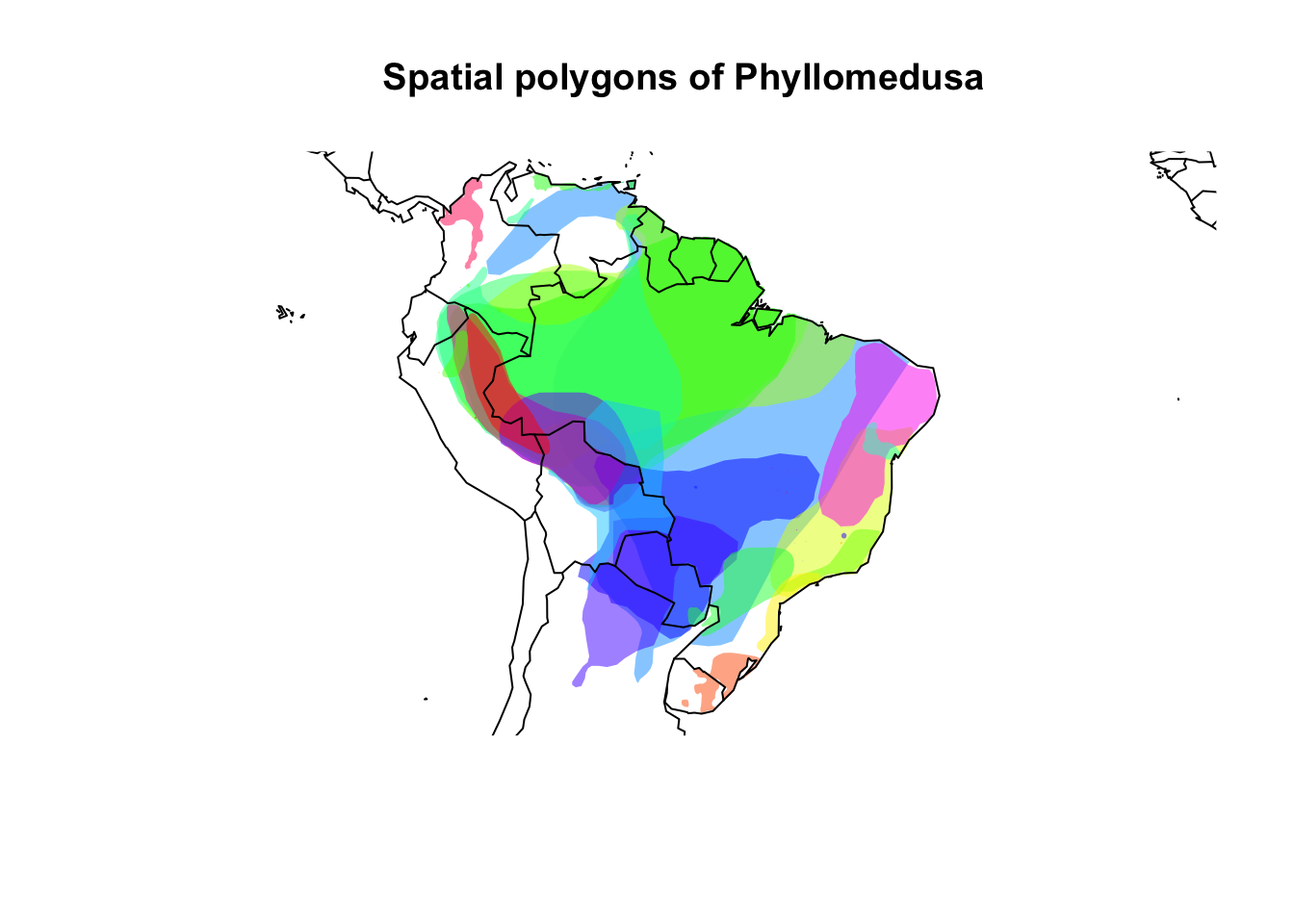
Quick start
Next step we can use the function lets.presab to convert species’ ranges (in shapefile format) into a presence-absence matrix based on a user-defined grid system. A simple way to do this is to define the extent and resolution of the grid.
PAM <- lets.presab(Phyllomedusa, xmn = -93, xmx = -29,
                   ymn = -57, ymx = 15, res = 1)
Note that if you have shapefiles with more species, or if you decide for a high resolution grid, the function may run very slowly. In this case, you may want to keep track of the analysis relative running time by setting the argument count = TRUE.
The lets.presab returns a PresenceAbsence object (unless show.matrix = TRUE, which in this case only a presence absence matrix is returned). The PresenceAbsence object is basically a list containing a presence absence matrix, a raster with the geographical information, and the species names (for more information ?PresenceAbsence). We can use the function summary to generate summary data about the PAM we just created.
summary(PAM)##
## Class: PresenceAbsence
## _ _
## Number of species: 32
## Number of cells: 1168
## Cells with presence: 1168
## Cells without presence: 0
## Species without presence: 0
## Species with the largest range: Phyllomedusa hypochondrialis
## _ _
## Grid parameters
## Resolution: 1, 1 (x, y)
## Extention: -93, -29, -57, 15 (xmin, xmax, ymin, ymax)
## Coord. Ref.: +proj=longlat +datum=WGS84 +ellps=WGS84 +towgs84=0,0,0You can also use the plot function directly to the PAM object.
plot(PAM)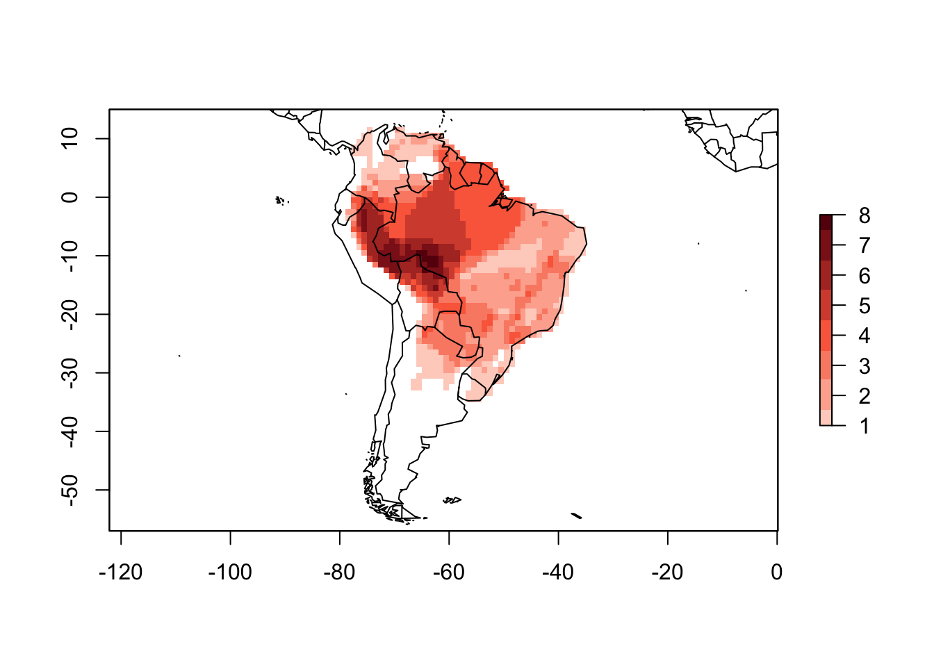
The plot function also allow users to plot specific species distributions. For example, we can plot the map of Phyllomedusa hypochondrialis:
plot(PAM, name = "Phyllomedusa hypochondrialis")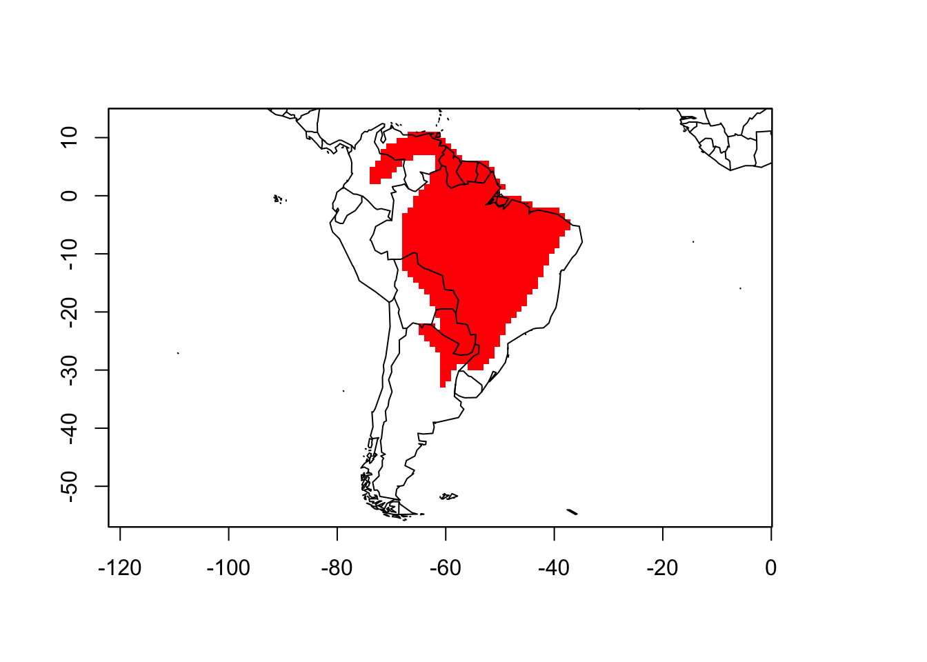
As I said before, the PAM object contains the actual presence absence matrix, to access it we can use the following code:
presab <- PAM$PThe first two columns of the matrix contain the longitude (x) and latitude (y) of the cells’ centroid, the following columns include the species’ presence(1) and absence(0) information.
# Print only the first 5 rows and 3 columns
presab[1:5, 1:3]
## Longitude(x) Latitude(y) Phyllomedusa araguari
## [1,] -74.5 11.5 0
## [2,] -69.5 11.5 0
## [3,] -68.5 11.5 0
## [4,] -75.5 10.5 0
## [5,] -74.5 10.5 0Using different projections
Some users may want to use different projections to generate the presence absence matrix. The lets.presab function allow users to do it by changing the crs.grid argument. Check the example using the South America Equidistant Conic projection.
pro <- paste("+proj=eqdc +lat_0=-32 +lon_0=-60 +lat_1=-5",
             "+lat_2=-42 +x_0=0 +y_0=0 +ellps=aust_SA",
             "+units=m +no_defs")
SA_EC <- CRS(pro)
PAM_proj <- lets.presab(Phyllomedusa, xmn = -4135157,
                        xmx = 4707602,
                        ymn = -450000, ymx = 5774733,
                        res = 100000,
crs.grid = SA_EC)summary(PAM_proj)##
## Class: PresenceAbsence
## _ _
## Number of species: 32
## Number of cells: 1376
## Cells with presence: 1376
## Cells without presence: 0
## Species without presence: 0
## Species with the largest range: Phyllomedusa hypochondrialis
## _ _
## Grid parameters
## Resolution: 1e+05, 1e+05 (x, y)
## Extention: -4135157, 4664843, -425267, 5774733 (xmin, xmax, ymin, ymax)
## Coord. Ref.: +proj=eqdc +lat_0=-32 +lon_0=-60 +lat_1=-5 +lat_2=-42 +x_0=0 +y_0=0 +ellps=aust_SA +units=m +no_defsplot(PAM_proj)
# Add projected country boundaries
library(maptools)
data("wrld_simpl")
world <- spTransform(wrld_simpl, SA_EC)
plot(world, add = TRUE)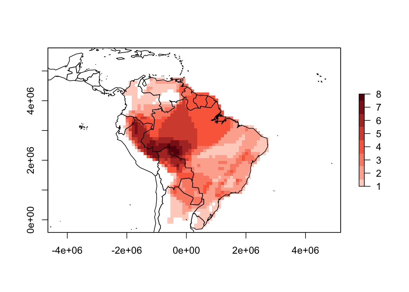
Note that I changed the extent and resolution parameters to match the new projection. A good way to determine both the extent and the resolution is to first transform the projection of a raster from a non-projected PresenceAbsence object, and see how the parameters changed. For example:
pr2 <- projectRaster(PAM$Richness_Raster, crs = SA_EC)
mean(res(pr2)) # Resolution value
## [1] 104900extent(pr2) # Extent values (i.e. xmn, xmx, ymn, ymx)## class : Extent
## xmin : -4716700
## xmax : 4471700
## ymin : -3568248
## ymax : 5755752Also note that the function assumes that the shapefiles are in WGS84 format, if this is not the case for your data you should change the crs argument.
Other features
The function lets.presab has some other useful arguments. For example, some users may want to exclude parts of the range where the species are extinct, or only keep the breeding ranges. The arguments presence, origin and seasonal allow users to filter the species distribution according to the IUCN classification of the different parts of a species range distribution. The specific values to use in these arguments may be obtained from the IUCN metadata files.
In some situations it is useful to only consider a species present in a cell if it covers more than a certain percentage value. Users can change this value using the argument cover. Note that this option is only available when the coordinates are in degrees (longitude/latitude). UPDATE: the version on github now allow users to use the argument cover with other projections.
# 90% cover
PAM_90 <- lets.presab(Phyllomedusa, xmn = -93,
                      xmx = -29, ymn = -57,
                      ymx = 15, res = 1,
                      cover = 0.9)
plot(PAM_90)
You can see now in the plot above that the cells close to the border of the continent do not indicate the presence of the species anymore.
When creating multiple PresenceAbsence objects for different groups, users may want to keep the same grid. In this case it is important to keep the argument remove.cells = FALSE, to avoid altering the grid. When remove.cells = TRUE the final matrix will not contain cells in the grid with a value of zero (i.e. sites with no species present).
PAM_keep_cells <- lets.presab(Phyllomedusa, xmn = -93,
                              xmx = -29, ymn = -57,
                              ymx = 15, res = 1,
                              remove.cells = FALSE)
Now you can use the summary function to verify if the empty cells were kept.
summary(PAM_keep_cells)##
## Class: PresenceAbsence
## _ _
## Number of species: 32
## Number of cells: 4608
## Cells with presence: 1168
## Cells without presence: 3440
## Species without presence: 0
## Species with the largest range: Phyllomedusa hypochondrialis
## _ _
## Grid parameters
## Resolution: 1, 1 (x, y)
## Extention: -93, -29, -57, 15 (xmin, xmax, ymin, ymax)
## Coord. Ref.: +proj=longlat +datum=WGS84 +ellps=WGS84 +towgs84=0,0,0Also, if users want to keep the species that do not occur in any cell of the grid it is necessary to set remove.sp = FALSE.
BirdLife shapefiles
BirdLife species distribution data can be slightly different from the ones provided by IUCN. The main difference is that they are normally provided in separated shapefiles, rather than in one unique shapefile containing all the species. letsR contains a specific function to deal with this kind of data. The function lets.presab.birds is an analogous function to lets.presab. The difference is that instead of a shapefile, users have to provide the path pointing to the location of all birds shapefiles. In the example below we will build a PresenceAbsence object to Ramphastos birds.
# Attention: For your own files change the path.
path_Ramphastos <- system.file("extdata", package = "letsR")
PAM_birds <- lets.presab.birds(path_Ramphastos, xmn = -93, xmx = -29,
                               ymn = -57, ymx = 25)
We can also use the functions summary and plot to the result of lets.presab.birds.
summary(PAM_birds)##
## Class: PresenceAbsence
## _ _
## Number of species: 11
## Number of cells: 1173
## Cells with presence: 1173
## Cells without presence: 0
## Species without presence: 0
## Species with the largest range: Ramphastos culminatus
## _ _
## Grid parameters
## Resolution: 1, 1 (x, y)
## Extention: -93, -29, -57, 25 (xmin, xmax, ymin, ymax)
## Coord. Ref.: NAplot(PAM_birds)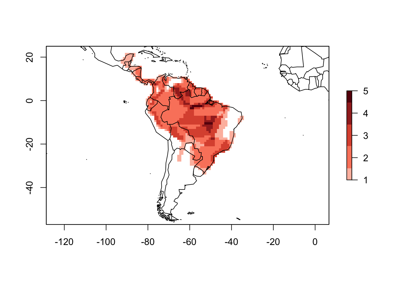
All the options in lets.presab are also available in lets.presab.birds.
Occurrence data (e.g. GBIF)
Another common source of spatial data are occurrence records. The function lets.presab.points allows users to input occurrence records to generate a PresenceAbsence object. To use this function you will need a two column matrix with longitude and latitude, and a vector indicating the species name of each occurrence record. The example below uses occurrence data from GBIF for Phyllomedusa, obtained using the R package spocc.
library(spocc)# Get occurrences for Phyllomedusa
occurrrences <- occ(query = 'Phyllomedusa', from = 'gbif', limit = 5000)
data <- occurrrences$gbif$data$Phyllomedusa
# Remove NAs
remove_na <- is.na(data$longitude) | is.na(data$latitude)
data <- data[!remove_na, ]
xy <- data[, c("longitude", "latitude")] # coordinates
sp_name <- data$nameNow that we have the coordinates and species name, we can use the lets.presab.points function.
PAM_points <- lets.presab.points(xy, sp_name, xmn = -93, xmx = -29,
                                 ymn = -57, ymx = 15, res = 1)
plot(PAM_points)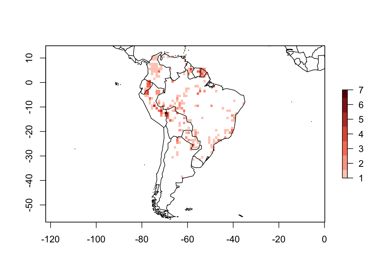
Using your own grid
For different reasons some users may want to create a presence absence matrix based on their own grid in shapefile format. The function lets.presab.grid allow users to convert species’ ranges into a presence-absence matrix based on a grid in shapefile format. However, this function only returns the actual matrix of presence absence and the grid, not an PresenceAbsence object. In some situations it is possible to convert this result to a PresenceAbsence object, I will cover this in a new post soon. Let’s first create our grid:
# Grid
sp.r <- rasterToPolygons(raster(xmn = -93, xmx = -29,
                                ymn = -57, ymx = 15,
                                resolution = 5))
# Give an ID to the cell
slot(sp.r, "data") <- cbind("ID" = 1:length(sp.r),
                            slot(sp.r, "data"))
plot(sp.r, border = rgb(.5, .5, .5))
map(add = T)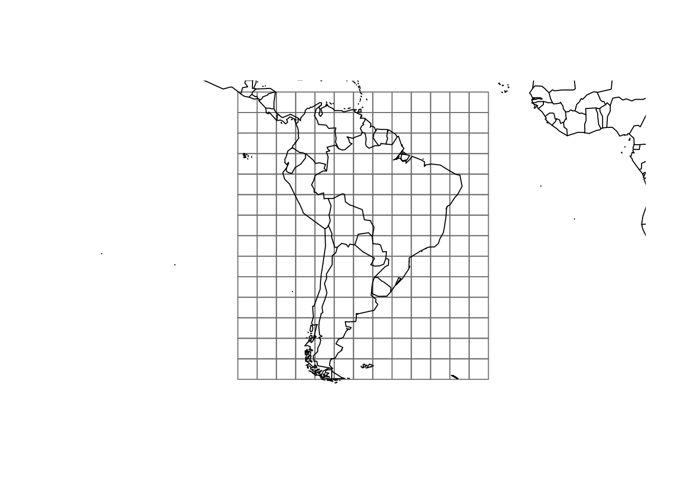
The grid and the species ranges should be in the same projection.
data(Phyllomedusa)
projection(Phyllomedusa) <- projection(sp.r)
Now we can build our presence absence matrix from the grid.
resu <- lets.presab.grid(Phyllomedusa, sp.r, "ID")The result is a list with the presence absence matrix and the grid. To plot the richness map we can use the following code:
rich_plus1 <- rowSums(resu$PAM) + 1
colfunc <- colorRampPalette(c("#fff5f0", "#fb6a4a", "#67000d"))
colors <- c("white", colfunc(max(rich_plus1)))
plot(resu$grid, border = "gray40",
     col = colors[rich_plus1])
map(add = TRUE)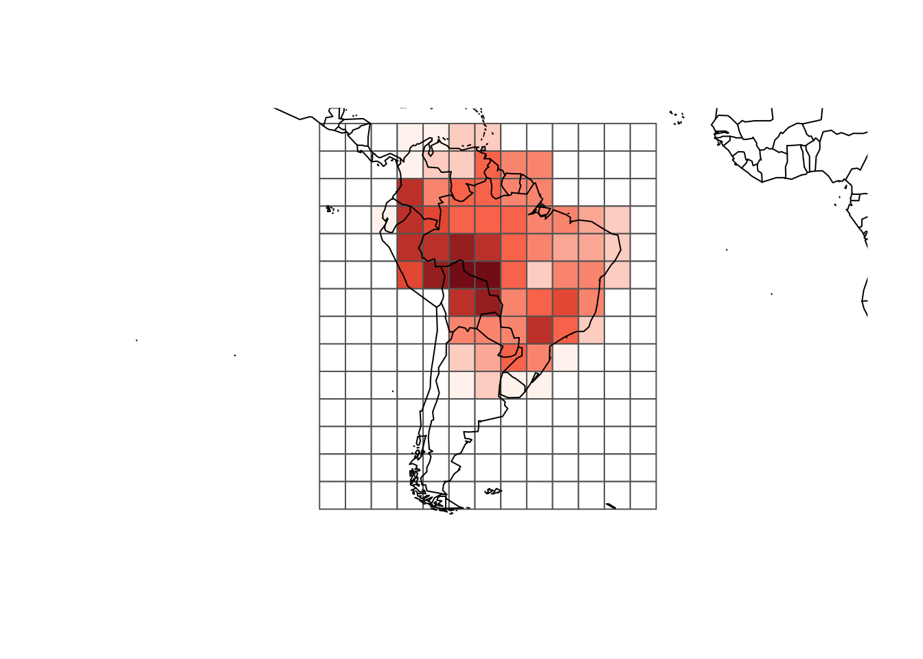
This covers all the functions to convert species distribution into presence absence matrix using the letsR package. Let me know if you have any suggestion or comments, and please share if you like it.
To cite letsR in publications use: Bruno Vilela and Fabricio Villalobos (2015). letsR: a new R package for data handling and analysis in macroecology. Methods in Ecology and Evolution. DOI: 10.1111/2041-210X.12401