Most of letsR package functions require a PresenceAbsence object (see previous post). But some users may already have a matrix of species presence absence (PAM) generated somewhere else or created using the lets.presab.grid function. In this post I will show how to transform these PAM files into a PresenceAbsence object.
First, note that this will only be possible if your grid used to generate the PAM is a square or a rectangular grid. Most of letsR functions are based on raster files, and rasters can only be square or rectangular.
So, first I will generate an example file using the function lets.presab.grid.
library(letsR)sp.r <- rasterToPolygons(raster(xmn = -93, xmx = -29,
ymn = -57, ymx = 15,
resolution = 5))
# Give an ID to the cell
slot(sp.r, "data") <- cbind("ID" = 1:length(sp.r),
slot(sp.r, "data"))
data(Phyllomedusa)
projection(Phyllomedusa) <- projection(sp.r)
resu <- lets.presab.grid(Phyllomedusa, sp.r, "ID")
rich_plus1 <- rowSums(resu$PAM) + 1
colfunc <- colorRampPalette(c("#fff5f0", "#fb6a4a", "#67000d"))
colors <- c("white", colfunc(max(rich_plus1)))
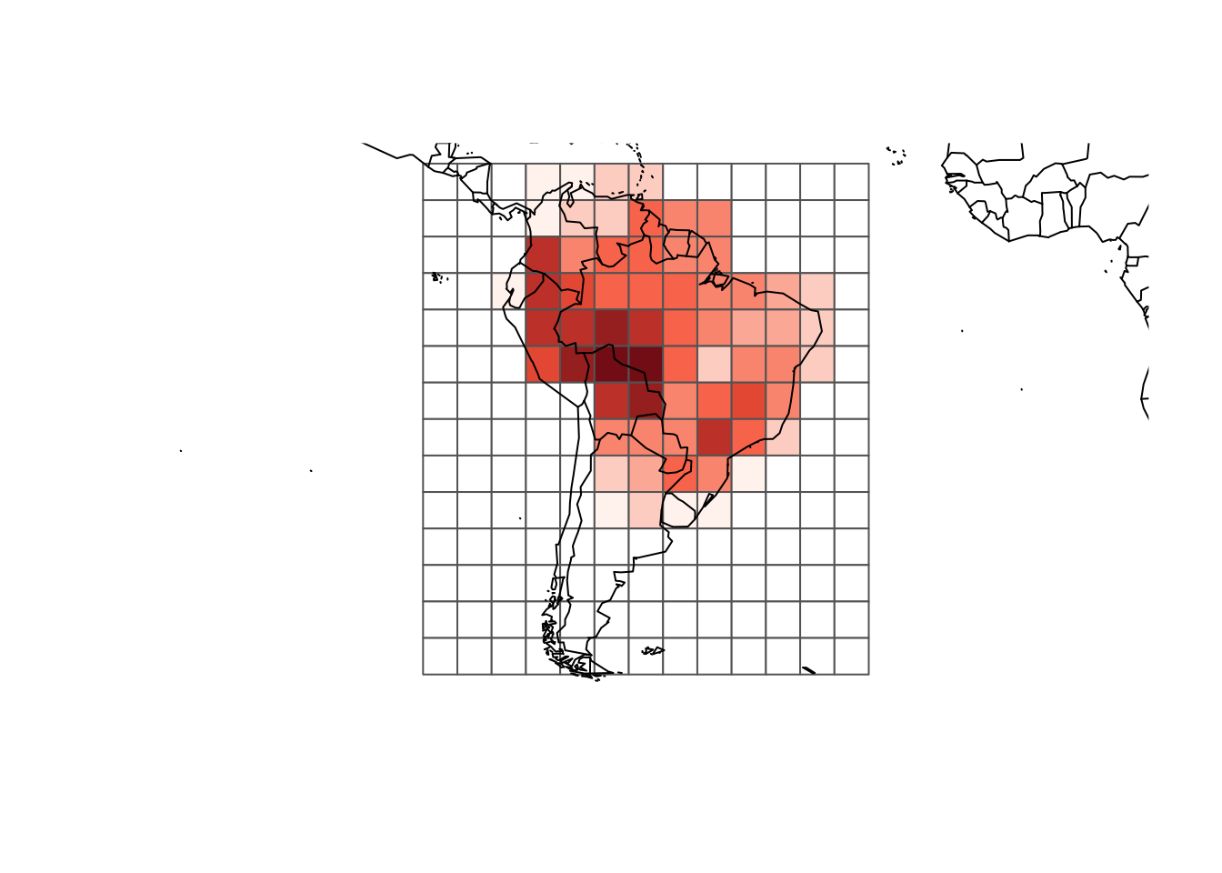
plot(resu$grid, border = "gray40",
col = colors[rich_plus1])
map(add = TRUE)
Now we have a PAM in matrix format, with the row names indicating the cell ID in a gird.
# Print only te first rows and columns of the PAM
resu$PAM[1:5, 1:3]
## Phyllomedusa atelopoides Phyllomedusa iheringii Phyllomedusa distincta
## 1 0 0 0
## 2 0 0 0
## 3 0 0 0
## 4 0 0 0
## 5 0 0 0And we also have a grid.
resu$grid## class : SpatialPolygonsDataFrame
## features : 182
## extent : -93, -28, -55, 15 (xmin, xmax, ymin, ymax)
## coord. ref. : +proj=longlat +datum=WGS84 +ellps=WGS84 +towgs84=0,0,0
## variables : 2
## names : ID, layer
## min values : 1, Inf
## max values : 182, -InfWe have to first transform the grid into a raster file. To do this, you have to know the resolution and extent of your grid. In this case the resolution is 5, and we can get the extent direct from the grid.
ext <- extent(resu$grid)
xmn <- ext[1]
xmx <- ext[2]
ymn <- ext[3]
ymx <- ext[4]

r <- raster(resolution = 5, xmn = xmn, xmx = xmx,
            ymn = ymn, ymx = ymx)
rich <- rasterize(resu$grid, r, field = "ID")
values(rich) <- rowSums(resu$PAM)
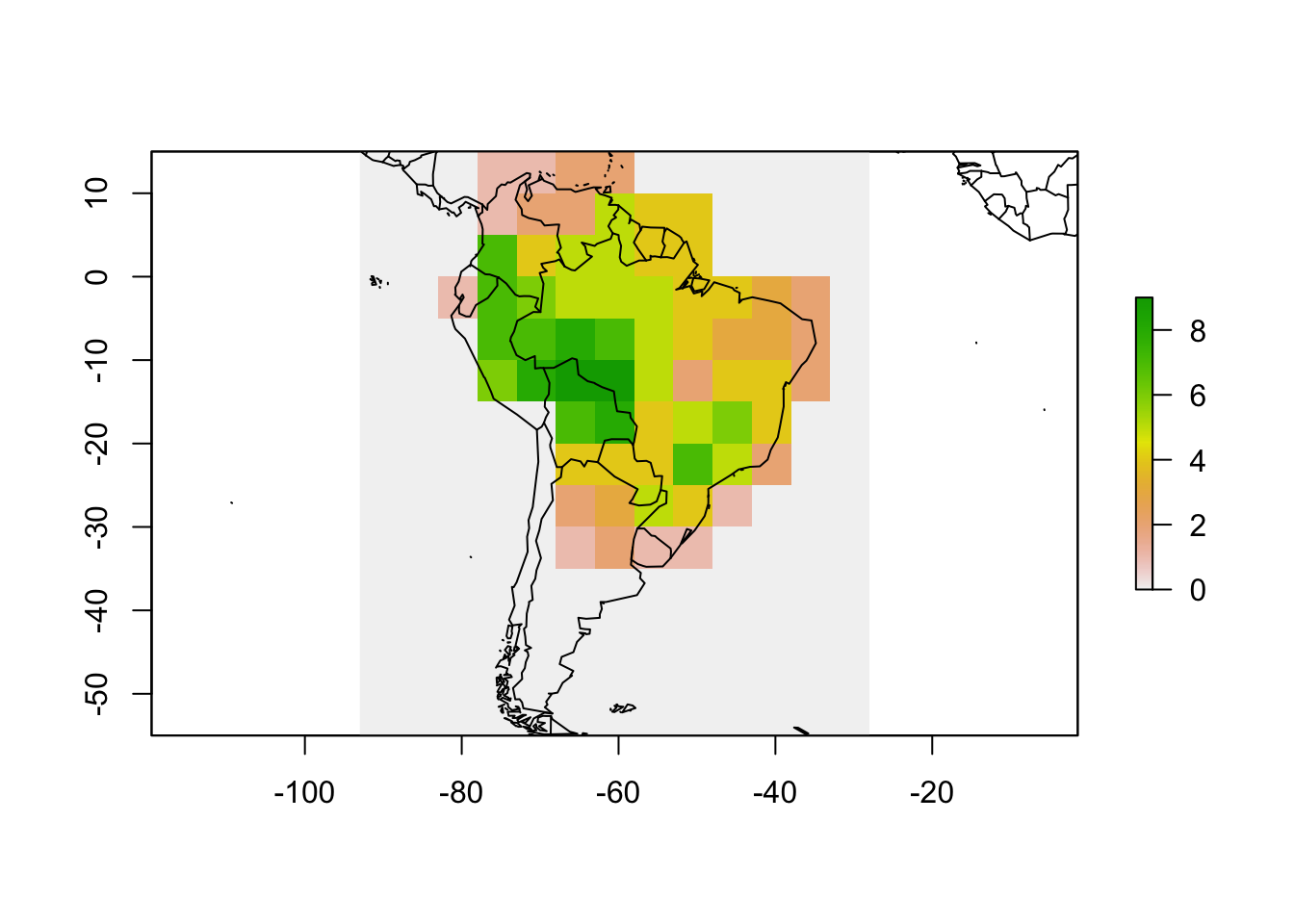
plot(rich)
map(add = TRUE)
Now the grid is in a raster format and contains species richness values, which is one of the objects of the PresenceAbsence object. We can now make the other two.
xy <- xyFromCell(rich, 1:ncell(rich))
colnames(xy) <- c("Longitude(x)", "Latitude(y)")
pam <- cbind(xy, resu$PAM)
pam[1:5, 1:3] # print first 3 columns and 5 rows
## Longitude(x) Latitude(y) Phyllomedusa atelopoides
## 1 -90.5 12.5 0
## 2 -85.5 12.5 0
## 3 -80.5 12.5 0
## 4 -75.5 12.5 0
## 5 -70.5 12.5 0species_names <- colnames(resu$PAM)We also have the PAM with the centroid of the cells and the species name file. We are ready to make the PresenceAbsence object.
PAM_from_grid <- list(pam, rich, species_names)
data("PAM")
names(PAM_from_grid) <- names(PAM)
class(PAM_from_grid) <- class(PAM)
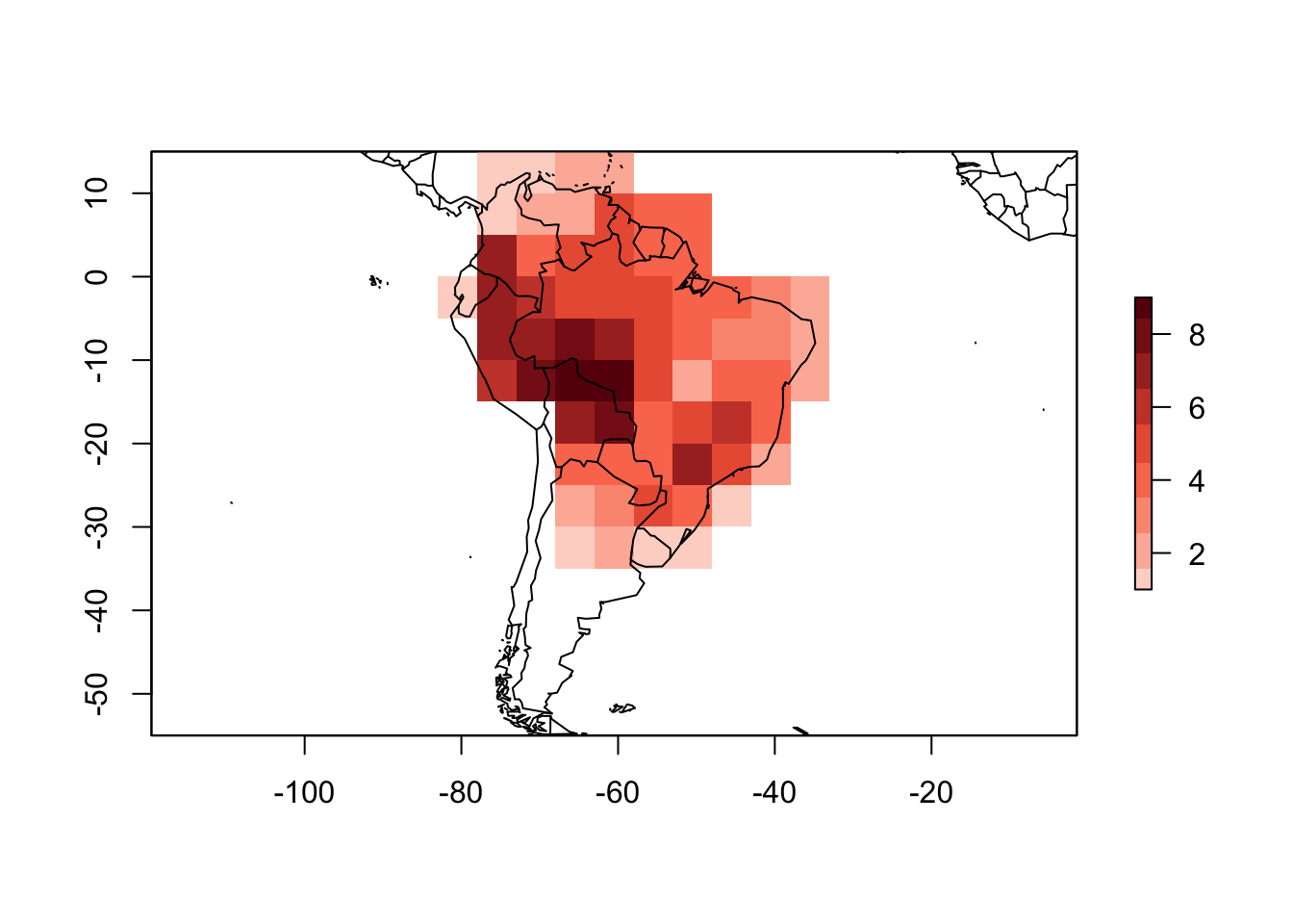
The transformation is complete. Now we can use all the methods for a PresenceAbsence object.
summary(PAM_from_grid)##
## Class: PresenceAbsence
## _ _
## Number of species: 23
## Number of cells: 182
## Cells with presence: 65
## Cells without presence: 117
## Species without presence: 0
## Species with the largest range: Phyllomedusa hypochondrialis
## _ _
## Grid parameters
## Resolution: 5, 5 (x, y)
## Extention: -93, -28, -55, 15 (xmin, xmax, ymin, ymax)
## Coord. Ref.: +proj=longlat +datum=WGS84 +ellps=WGS84 +towgs84=0,0,0plot(PAM_from_grid)
To cite letsR in publications use: Bruno Vilela and Fabricio Villalobos (2015). letsR: a new R package for data handling and analysis in macroecology. Methods in Ecology and Evolution. DOI: 10.1111/2041-210X.12401