Many times scientists are interested in analyzing or describing the geographical variation of a trait. For example, how species body size varies across the space. Here I will show how to map species traits using the letsR package.
To do this, let’s test the Rapoport’s rule on Phyllomedusa frogs. Following Wikipedia: “Rapoport’s rule is an ecogeographical rule that states that latitudinal ranges of plants and animals are generally smaller at lower latitudes than at higher latitudes.”.
To start this test we can load our PresenceAbsence object that we generated previously (see the first and second posts on how to do it).
Note: I recommend to use the latest version of the letsR package on GitHub
library(letsR)data("PAM")
# Change the color
cols <- colorRampPalette(c('#ffffd9','#edf8b1','#c7e9b4',
'#7fcdbb','#41b6c4',
'#1d91c0','#225ea8'))
plot(PAM, col_rich = cols)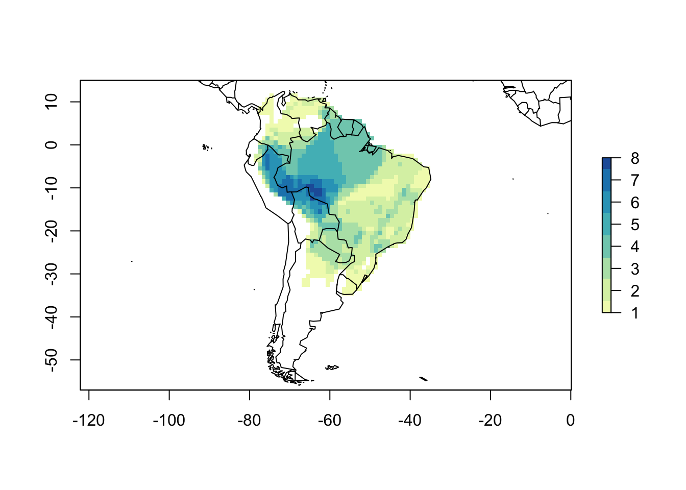
Now, we have to calculate the species range sizes. letsR includes a function to do that called lets.rangesize. We can calculate the range size from the PresenceAbsence matrix, as the number of cells or in square meters. Alternatively, we can do it directly on the species ranges shapefiles. Let’s do the latter option, since it is more accurate, although all options should be correlated.
data("Phyllomedusa")
rangesize <- lets.rangesize(Phyllomedusa,
                            coordinates = "geographic")
rangesize <- rangesize / 1000 # Transform in km2
Community level analysis
To map this trait by cell, we can use the lets.maplizer function. You can choose the function to aggregate the species trait per cell, but in this case we want to use the default option that will average the values. We also want the function to return a raster with the mapped traits, so we will set ras = TRUE.
resu <- lets.maplizer(PAM, rangesize, rownames(rangesize), ras = TRUE)
cols2 <- colorRampPalette(c('#e0ecf4','#9ebcda','#8856a7'))
plot(resu$Raster, col = cols2(10), main = "Mean Range Size")
map(add = TRUE)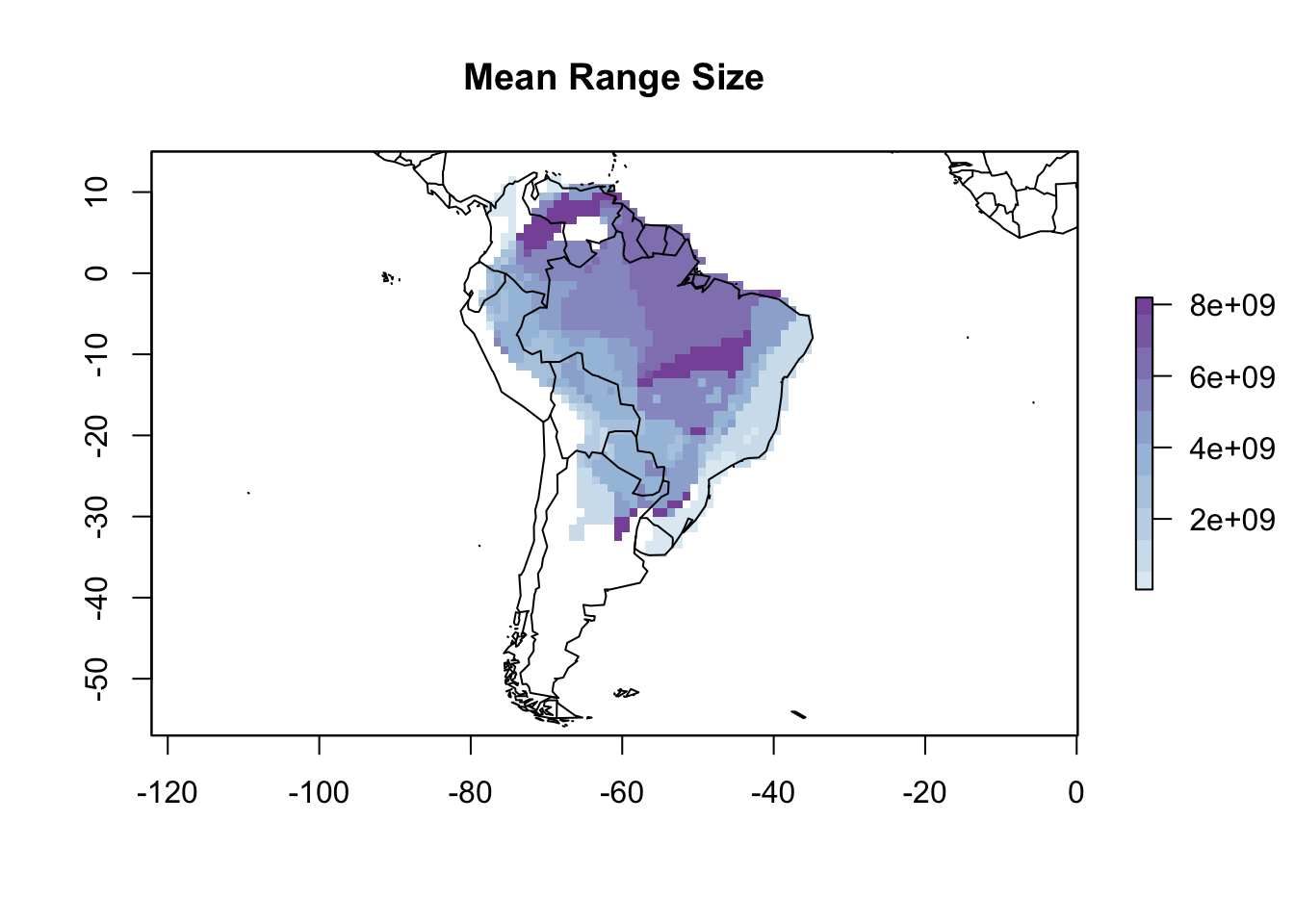
Visually, the Rapoport’s rule doesn’t seem to work on Phyllomedusa frogs. We can go further and see the relationship with latitude.
library(ggplot2)mpg <- as.data.frame(resu$Matrix)
f <- ggplot(mpg, aes(`Latitude(y)`, Variable_mean))
f + geom_smooth(model = lm) +
geom_point(col = rgb(0, 0, 0, .6)) +
labs(y = "Range Size") +
theme_bw()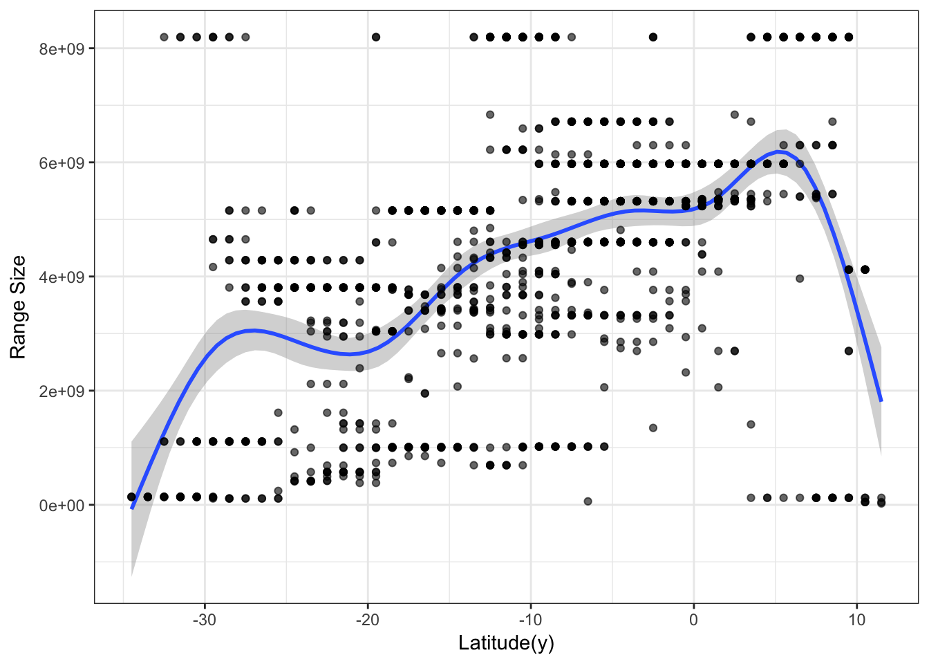
Seems that the Rapoport’s rule doesn’t stand for this genus, actually the direction seems inverted, at least when analyzing it at the community level. However, to confirm this we would have to perform formal statistical analysis and control for spatial autocorrelation problems.
A quick note here. Scientists should be carefull with this type of comunity analysis, as the repetition in species co-occurrence can easilly generate spourious patterns and significant correlations (see our paper for further discussion).
To cite letsR in publications use: Bruno Vilela and Fabricio Villalobos (2015). letsR: a new R package for data handling and analysis in macroecology. Methods in Ecology and Evolution. DOI: 10.1111/2041-210X.12401