This is an updated version of the code description found in the supplementary matterial of the manuscript “Contextualized niche shifts upon independent invasions by the dung beetle Onthophagus taurus” by Daniel Silva, Bruno Vilela, Bruno Buzatto, Armin Moczek and Joaquin Hortal. Note that due to some packages and analysis updates some values and figures may be different from the original results.
About
This document serves as a guide to reproduce the analyzes and results presented in the manuscript: “Contextualized niche shifts upon independent invasions by the dung beetle Onthophagus taurus” by Daniel Silva, Bruno Vilela, Bruno Buzatto, Armin Moczek and Joaquin Hortal.
The objective of this document is to record the code used to generate the results and allow the readers to better explore the possibilities of the research.
This document was written in R markdown format, which allows the use of easy-formatting plain text with R code chunks. For more information see the package knitr (http://yihui.name/knitr/).
Before starting
Prior to the analyzes, we recommend all users to check the latest version of R at http://www.r-project.org/ and to make sure that they are using the updated versions of their installed R packages. Users can automatically update their installed packages with the following code:
# Update installed packages
update.packages(checkBuilt = TRUE, ask = FALSE)
The analysis presented here makes use of the following R packages available at CRAN. Use the following code to install them.
# Install packages
install.packages("knitr")
install.packages("spThin")
install.packages("rgeos")
install.packages("sp")
install.packages("maptools")
install.packages("raster")
install.packages("ecospat")
Once installed, load them.
# Load packages
library(knitr)
library(spThin)
library(rgeos)
library(sp)
library(maptools)
library(raster)
library(ecospat)
Data
Load the occurrence records
Place the file containing the occurrence records (file points.txt) in your work directory (use getwd() to check your work directory). The next step is to load the occurrence records into the R environment.
occ.points <- read.table("points.txt", sep = "\t", header = TRUE)The loaded table includes 1272 occurrence records.
Thining occurrence records
The occurrence records gathered (see the methods section of the manuscript, for the description of how we obtained the data) are not free from geographical sample bias. To minimize this problem, we applied a thinning procedure using the spThin package to make sure that all the points have at least a minimum distance of 10km from each other (see Aiello-Lammens et al. 2014 for the algorithm description).
occ.points.thin <- thin(occ.points, verbose = FALSE,
                        lat.col = "Latitude",
                        long.col = "Longitude",
                        spec.col = "Scientific.name",
                        thin.par = 10,
                        reps = 1,
                        write.files = FALSE,
                        write.log.file = FALSE,
                        locs.thinned.list.return = TRUE)
After the thinning procedure the number of occurrence points is reduced to n = 1059.
To check the distribution of the occurrence records we map them in a world context.
data(wrld_simpl)
plot(wrld_simpl)
points(occ.points.thin[[1]], col = "purple", pch = 20, cex = 0.7)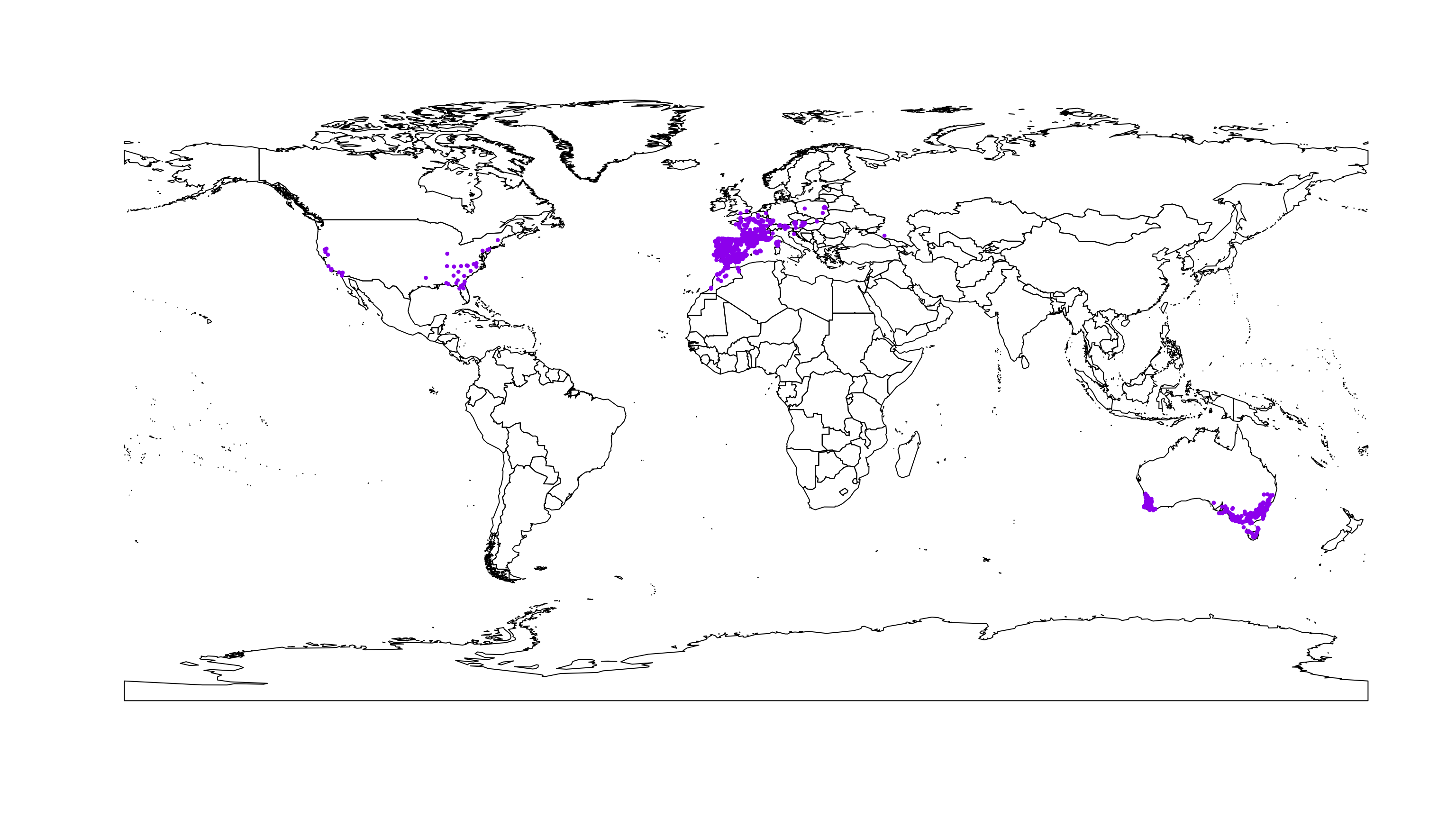
Define the regions to be tested
The “niche” comparisons can be done between any group of occurrence points defined. For example, the groups can be divided into major regions, e.g. native occurrence (Europe and North Africa), Australia and North America, or each region can be divided into more sub-regions, e.g. Western North America and Eastern North America. We left the option here for the readers to define their own regions and explore the results. In the following analyzes we decided to divide the occurrence records into 5 groups: Native (Europe and North Africa), Western North America, Eastern North America, Western Australia and Eastern Australia. We choose these regions as we believe that their invasion history are different and independent (see details in the manuscript).
The first step is to define the number of groups (regions) to be tested. In the follow case we choose 5 groups.
n.groups <- 5 Now, it is necessary to define the longitude limits of the region. In this specific case, only the longitude is needed to separate the groups. Change the object limits to define other groups, note that the object must have the n.groups - 1 length.
limits <- c(-100, -50, 100, 125)
begin <- min(occ.points.thin[[1]][, 1]) - 10
end <- max(occ.points.thin[[1]][, 1]) + 10
group.long <- c(begin, limits, end)
Check the limits by plotting them.
plot(wrld_simpl)
points(occ.points.thin[[1]], col = "purple", pch = 20, cex = 0.7)
abline(v = group.long, lty = 2, col = "red", lwd = 2)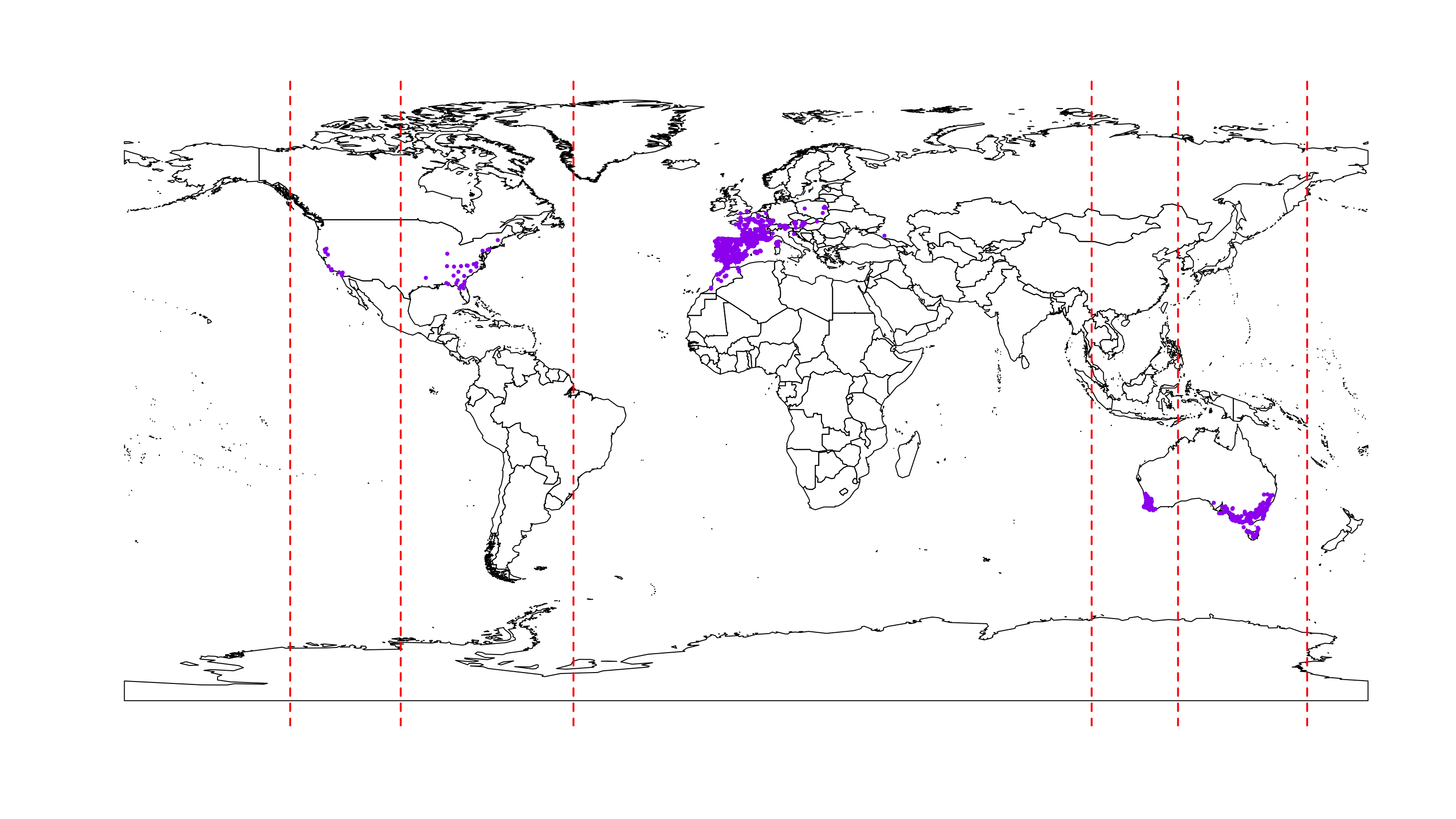
Now define the name of the groups, in the same geographical order of the groups, starting from the west to east. You can also define the codes to be used in the tables.
g.names <- c("Western North America",
             "Eastern North America",
             "Native",
             "Western Australia",
             "Eastern Australia")

g.codenames <- c("WestNorAme", "EastNorAme", "Native", "WestAus", "EastAus")
It is also necessary to set what colors will be used in the next plots for each group (using the same order as the names). Change the colors according to your preferences.
g.colors <- c("cyan", "darkblue", "red", "green", "darkgreen")Background definition
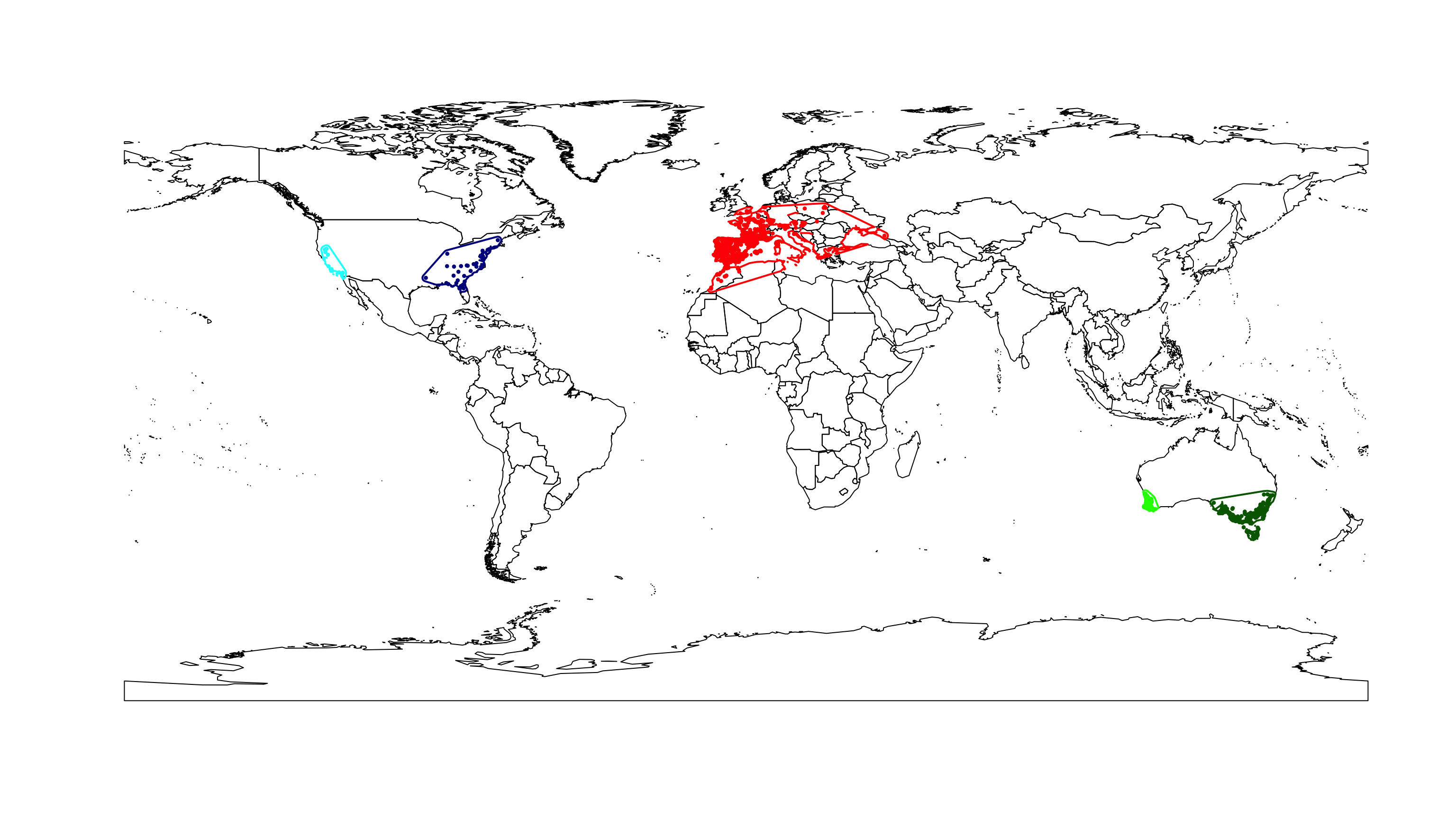
An important step in the niche analysis is the definition of the background. Here we applied a background based on a minimum convex polygon (MCP) made from the occurrence records of each group. Additionally to the MCP we add a buffer around it. The polygon buffer size for the background (in degrees) can be changed below. We chose 2 degrees based on the published values of dispersion for Onthophagus taurus (Hanski & Cambefort, 2014).
buffer.size <- 1We define a minimum convex polygon (MCP) function below (this function was obtained from https://github.com/ndimhypervol/wallace).
mcp <- function (xy) {
  xy <- as.data.frame(coordinates(xy))
  coords.t <- chull(xy[, 1], xy[, 2])
  xy.bord <- xy[coords.t, ]
  xy.bord <- rbind(xy.bord[nrow(xy.bord), ], xy.bord)
  return(SpatialPolygons(list(Polygons(list(Polygon(as.matrix(xy.bord))), 1))))
}
Enviromnental variables
The environmental variables used are available at the WorldClim website (http://www.worldclim.org). Download all the 19 bioclimatic (‘Biolclim’) variables for the current conditions (we used the resolution of 10 arc-min) with the code below. Note you need to have the internet on. The download files are opened directed in the R environment, but they are also saved in your work directory (to see where it is, use getwd()).
variables <- getData('worldclim', var='bio', res=10)In the manuscript we used the all the 19 bioclimatic variables as before the analysis we will reduce them to a two-dimensional space with a PCA. However, the readers can choose the number of variables to keep by changing the sequence 1:19 in the code below for the variable number you want to keep (to see the name sequence of the variables apply names(variables)).
variables <- subset(variables, 1:19)You can also check the variables, by mapping them.
plot(variables)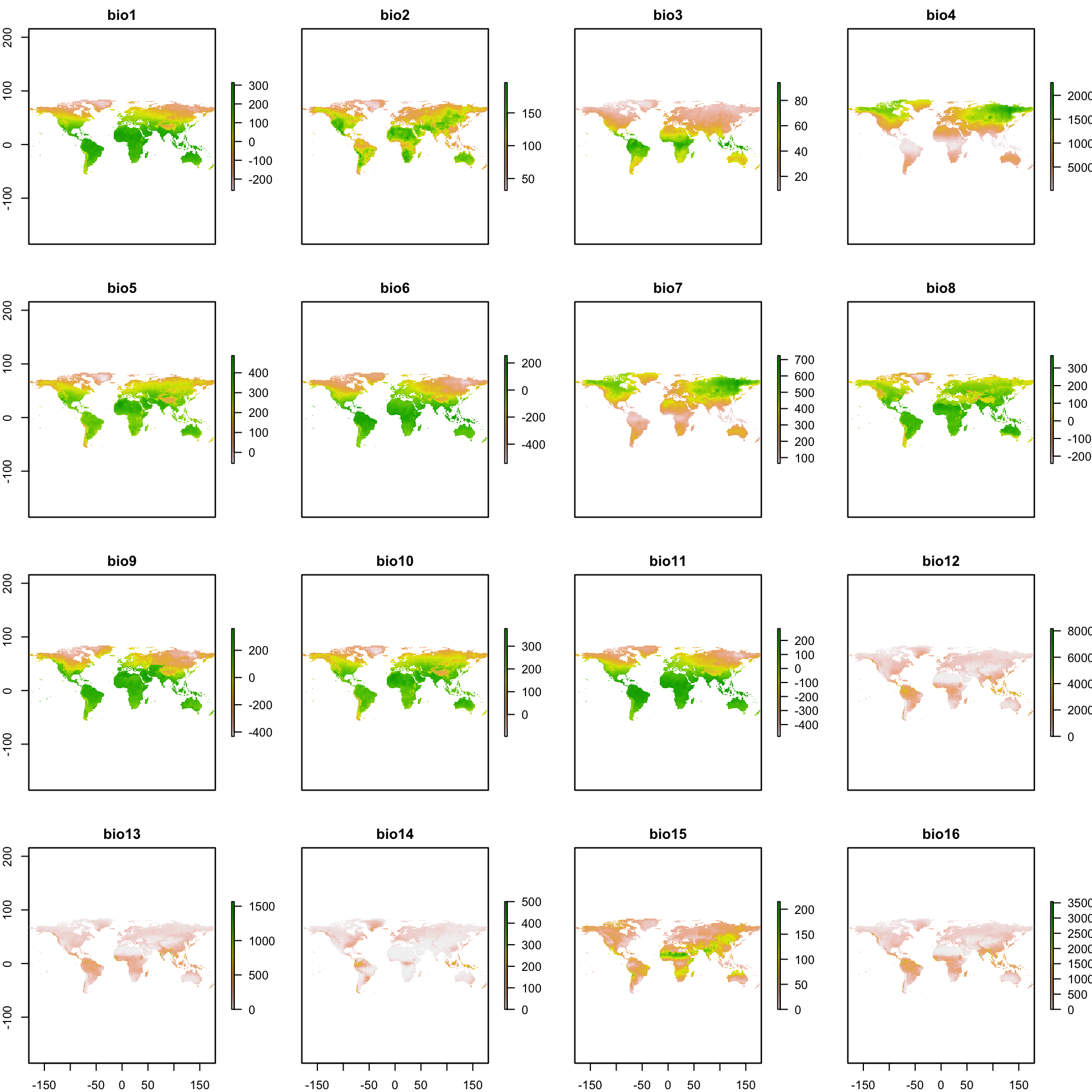
Group assigning
Once, we have the occurrence data, the environmental data, the defined groups and their background parameters chosen, we can prepare the data for the analysis. Below we use the occurrence points to generate the MCP plus a buffer defined by the user for the background (see above). Next, the variable values per group are extracted from the species occurrence points and from the background (defined above). Finally we plot the resulting groups with their respective backgrounds.
# Union of the world map
lps <- getSpPPolygonsLabptSlots(wrld_simpl)
IDFourBins <- cut(lps[,1], range(lps[,1]), include.lowest=TRUE)
world <- unionSpatialPolygons(wrld_simpl, IDFourBins)

# Empty objects
g.assign <- numeric(nrow(occ.points.thin[[1]]))
xy.mcp <- list()
back.env <- list()
spec.env <- list()
row.sp <- list()

# Plot map
plot(wrld_simpl)

# Loop
for(i in 1:n.groups) {

  # Define groups
  cut1 <- occ.points.thin[[1]][, 1] >= group.long[i]
  cut2 <- occ.points.thin[[1]][, 1] < group.long[i + 1]
  g.limit <- cut1 & cut2

  # Save row numbers per species
  row.sp[[i]] <- which(g.limit)
  g.assign[g.limit] <- g.names[i]

  # Background polygon
  mcp.occ <- mcp(as.matrix(occ.points.thin[[1]][g.limit, ]))
  xy.mcp.i <- gBuffer(mcp.occ, width = buffer.size)
  proj4string(xy.mcp.i) <- proj4string(world)
  xy.mcp[[i]] <- gIntersection(xy.mcp.i, world, byid=TRUE, drop_lower_td=TRUE)
  # Background environment
  back.env[[i]] <- na.exclude(do.call(rbind.data.frame, extract(variables, xy.mcp[[i]])))
  # Species environment
  spec.env[[i]] <- na.exclude(extract(variables, occ.points.thin[[1]][g.limit, ]))

  # Plot
  points(occ.points.thin[[1]][g.limit, ], col = g.colors[i],
         pch = 20, cex = 0.7)
  plot(xy.mcp[[i]], add = TRUE, border = g.colors[i], lwd = 2)

}
Now we organize the final tables to be used.
# Occurrence points per group
g.occ.points <- cbind("Groups" = g.assign, occ.points.thin[[1]])
# Environmental values for the background
all.back.env <- do.call(rbind.data.frame, back.env)
# Environmental values for the species occurrence points
all.spec.env <- do.call(rbind.data.frame, spec.env)
# Environmental values all together
data.env <- rbind(all.spec.env, all.back.env)
Check the number of occurrence records per region.
table(g.occ.points[, 1])Eastern Australia Eastern North America Native
164 29 786
Western Australia Western North America
69 11 Niche comparissons
The niche analyzes and comparisons follow the framework developed by Broennimann et al. (2012) and its derivations (see methods section in the manuscript).
PCA
We chose to apply a PCA (Principal Component Analysis) considering all the environments together, as it presented the best performance when comparing the niches (Broennimann et al., 2012).
# Weight matrix
w <- c(rep(0, nrow(all.spec.env)), rep(1, nrow(all.back.env)))
# PCA of all environment
pca.cal <- dudi.pca(data.env, row.w = w, center = TRUE,
                    scale = TRUE, scannf = FALSE, nf = 2)
Once we have the pca results, we need the first and second eigenvector values for the background and for the occurrence records per group.
# Rows in data corresponding to sp1
adtion <- cumsum(c(0, sapply(back.env, nrow)))
begnd <- nrow(all.spec.env)
# Empty list to save the results
scores.back <- list()
scores.spec <- list()

# Assigning the values
for (i in 1:n.groups) {
  scores.spec[[i]] <- pca.cal$li[row.sp[[i]], ]
  pos <- (begnd[1] + adtion[i] + 1) : (begnd[1] + adtion[i + 1])
  scores.back[[i]] <- pca.cal$li[pos, ]
}

total.scores.back <- do.call(rbind.data.frame, scores.back)
Environmental space
An environmental space is generated based on the pca values calculated for the background and the occurrence records. We defined the resolution of this two-dimensional space grid below.
R <- 100Next, we modeled the species density in the environmental grid, considering the observed occurrence density and the availability of the conditions in the background.
z <- list()

for (i in 1:n.groups) {
  z[[i]] <- ecospat.grid.clim.dyn(total.scores.back,
                                  scores.back[[i]],
                                  scores.spec[[i]],
                                  R = R)
}
Niche overlap
For the niche overlap, we calculate the D metric and its significance, using a similarity test. We define the number of interactions for the similarity test below (see the methods section in the manuscript for details).
rep <- 100Once the number of interactions is defined, we can generate the values. Additionally, we calculate the partition of the non-overlapped niche, among niche unfilling, expansion and stability (see methods in the manuscript).
# Empty matrices
D <- matrix(nrow = n.groups, ncol = n.groups)
rownames(D) <- colnames(D) <- g.codenames
unfilling <- stability <- expansion <- sim <- D

for (i in 2:n.groups) {

  for (j in 1:(i - 1)) {

    x1 <- z[[i]]
    x2 <- z[[j]]

    # Niche overlap
    D[i, j] <- ecospat.niche.overlap (x1, x2, cor = TRUE)$D

    # Niche similarity
    sim[i, j] <- ecospat.niche.similarity.test (x1, x2, rep,
                                                alternative = "greater")$p.D
    sim[j, i] <- ecospat.niche.similarity.test (x2, x1, rep,
                                                alternative = "greater")$p.D

    # Niche Expansion, Stability, and Unfilling
    index1 <- ecospat.niche.dyn.index (x1, x2,
                                       intersection = NA)$dynamic.index.w
    index2 <- ecospat.niche.dyn.index (x2, x1,
                                       intersection = NA)$dynamic.index.w
    expansion[i, j] <- index1[1]
    stability[i, j] <- index1[2]
    unfilling[i, j] <- index1[3]
    expansion[j, i] <- index2[1]
    stability[j, i] <- index2[2]
    unfilling[j, i] <- index2[3]
  }
}
Numeric results
Below we present the results for each metric, among all the groups.
D value:
kable(D, digits = 3, format = "markdown")| WestNorAme | EastNorAme | Native | WestAus | EastAus | |
|---|---|---|---|---|---|
| WestNorAme | NA | NA | NA | NA | NA |
| EastNorAme | 0.156 | NA | NA | NA | NA |
| Native | 0.386 | 0.160 | NA | NA | NA |
| WestAus | 0.241 | 0.167 | 0.182 | NA | NA |
| EastAus | 0.221 | 0.231 | 0.279 | 0.236 | NA |
Niche similarity null model (p-values):
kable(sim, digits = 3, format = "markdown")| WestNorAme | EastNorAme | Native | WestAus | EastAus | |
|---|---|---|---|---|---|
| WestNorAme | NA | 0.069 | 0.059 | 0.040 | 0.228 |
| EastNorAme | 0.089 | NA | 0.178 | 0.010 | 0.059 |
| Native | 0.030 | 0.139 | NA | 0.069 | 0.030 |
| WestAus | 0.020 | 0.010 | 0.030 | NA | 0.010 |
| EastAus | 0.168 | 0.030 | 0.030 | 0.010 | NA |
Niche Unfilling:
kable(unfilling, digits = 3, format = "markdown")| WestNorAme | EastNorAme | Native | WestAus | EastAus | |
|---|---|---|---|---|---|
| WestNorAme | NA | 0.541 | 0.260 | 0.486 | 0.224 |
| EastNorAme | 0.363 | NA | 0.291 | 0.888 | 0.342 |
| Native | 0.641 | 0.716 | NA | 0.845 | 0.334 |
| WestAus | 0.218 | 0.804 | 0.363 | NA | 0.326 |
| EastAus | 0.142 | 0.666 | 0.044 | 0.567 | NA |
Niche Expansion:
kable(expansion, digits = 3, format = "markdown")| WestNorAme | EastNorAme | Native | WestAus | EastAus | |
|---|---|---|---|---|---|
| WestNorAme | NA | 0.363 | 0.641 | 0.218 | 0.142 |
| EastNorAme | 0.541 | NA | 0.716 | 0.804 | 0.666 |
| Native | 0.260 | 0.291 | NA | 0.363 | 0.044 |
| WestAus | 0.486 | 0.888 | 0.845 | NA | 0.567 |
| EastAus | 0.224 | 0.342 | 0.334 | 0.326 | NA |
Niche Stability:
kable(stability, digits = 3, format = "markdown")| WestNorAme | EastNorAme | Native | WestAus | EastAus | |
|---|---|---|---|---|---|
| WestNorAme | NA | 0.637 | 0.359 | 0.782 | 0.858 |
| EastNorAme | 0.459 | NA | 0.284 | 0.196 | 0.334 |
| Native | 0.740 | 0.709 | NA | 0.637 | 0.956 |
| WestAus | 0.514 | 0.112 | 0.155 | NA | 0.433 |
| EastAus | 0.776 | 0.658 | 0.666 | 0.674 | NA |
Figure results
Individual niche plots
We developed some modifications in the plot.niche function available at Broennimann et al 2012. The modifications include more options and flexibility to the plot.
plot.niche.mod <- function(z, name.axis1 = "PC1", name.axis2 = "PC2",
                           cor = F, corte,  contornar = TRUE,
                           densidade = TRUE, quantis = 10,
                           back = TRUE, x = "red", title = "",
                           i) {


  cor1 <- function(cores.i, n) {
    al <- seq(0,1,(1/n))
    cores <- numeric(length(n))
    for(i in 1:n) {
      corespar <- col2rgb(cores.i)/255
      cores[i] <- rgb(corespar[1, ], corespar[2, ],
                      corespar[3, ], alpha = al[i])
    }
    return(cores)
  }


  a1 <- colorRampPalette(c("transparent",cor1(x, quantis)), alpha = TRUE)

  xlim <- c(min(sapply(z, function(x){min(x$x)})),
            max(sapply(z, function(x){max(x$x)})))

  ylim <- c(min(sapply(z, function(x){min(x$y)})),
            max(sapply(z, function(x){max(x$y)})))

  graphics::image(z[[1]]$x, z[[1]]$y, as.matrix(z[[1]]$z.uncor), col = "white",
                  ylim = ylim, xlim = xlim,
                  zlim = c(0.000001, max(as.matrix(z[[1]]$z.uncor), na.rm = T)),
                  xlab = "PC1", ylab = "PC2", cex.lab = 1.5,
                  cex.axis = 1.4)

  abline(h = 0, v = 0, lty = 2)

  if (back) {
    contour(z[[i]]$x, z[[i]]$y, as.matrix(z[[i]]$Z),
            add = TRUE, levels = quantile(z[[i]]$Z[z[[i]]$Z > 0],
                                          c(0, 0.5)), drawlabels = FALSE,
            lty = c(1, 2), col = x, lwd = 1)
  }

  if (densidade) {
    image(z[[i]]$x, z[[i]]$y, as.matrix(z[[i]]$z.uncor), col = a1(100), add = TRUE)
  }


  if(contornar){
    contour(z[[i]]$x, z[[i]]$y, as.matrix(z[[i]]$z.uncor),
            add = TRUE, levels = quantile(z[[i]]$z.uncor[z[[i]]$z.uncor > 0],
                                          seq(0, 1, (1 / quantis))),
            drawlabels = FALSE, lty = c(rep(2,(quantis - 1)), 1),
            col = cor1(x, quantis), lwd = c(rep(1, (quantis - 1)), 2))
  }

  title(title)
  box()
}
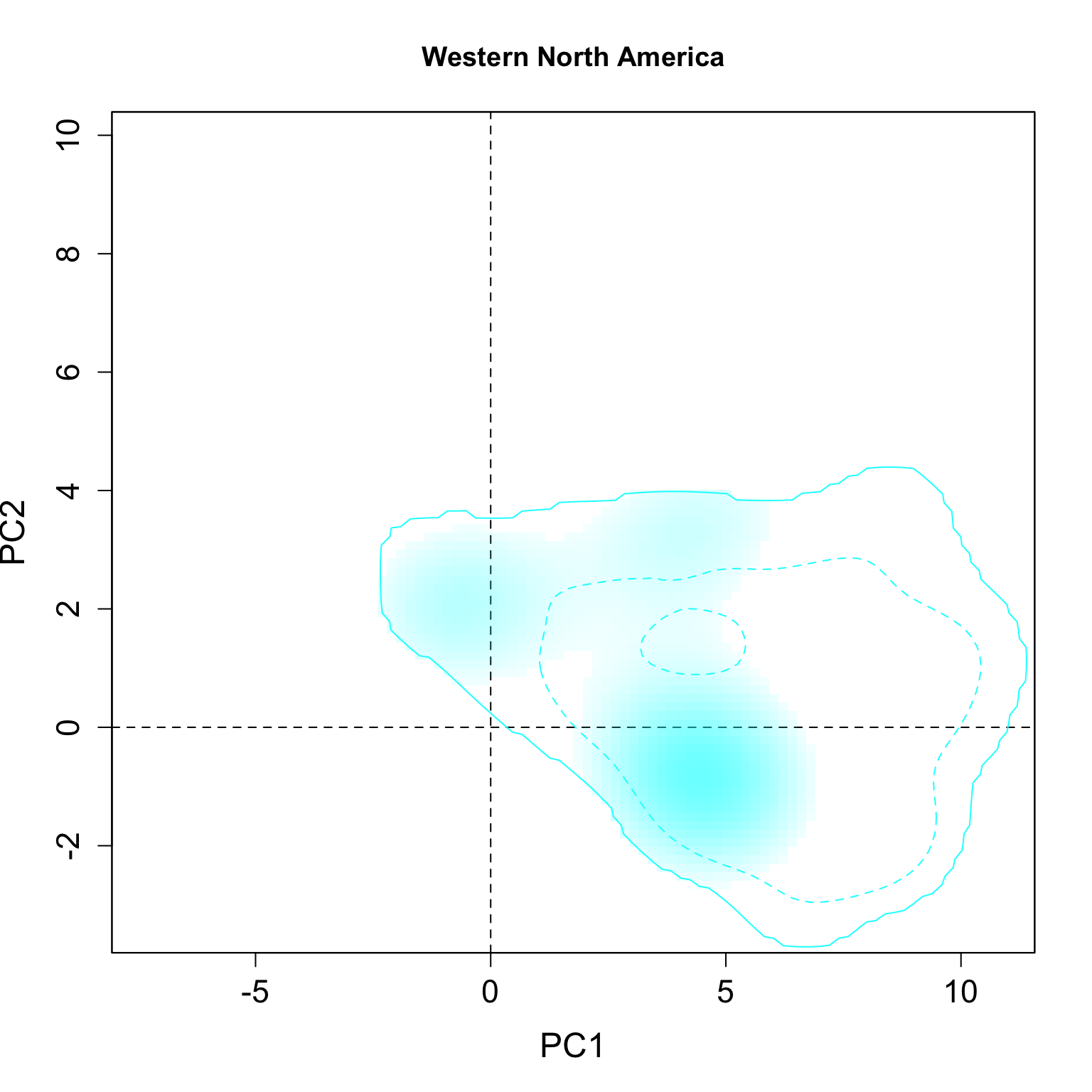
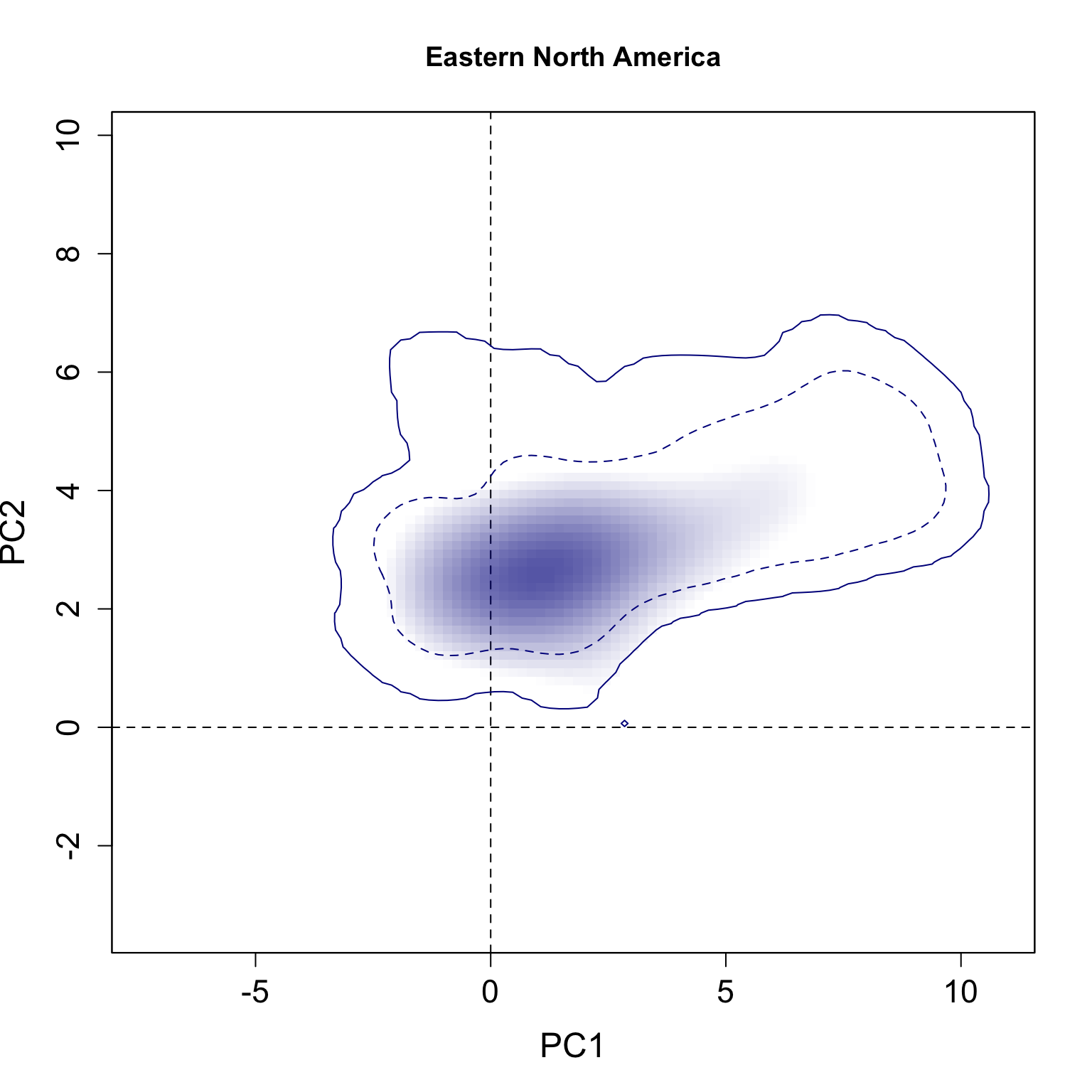
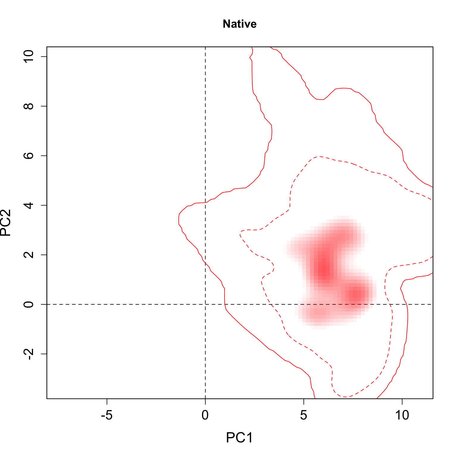
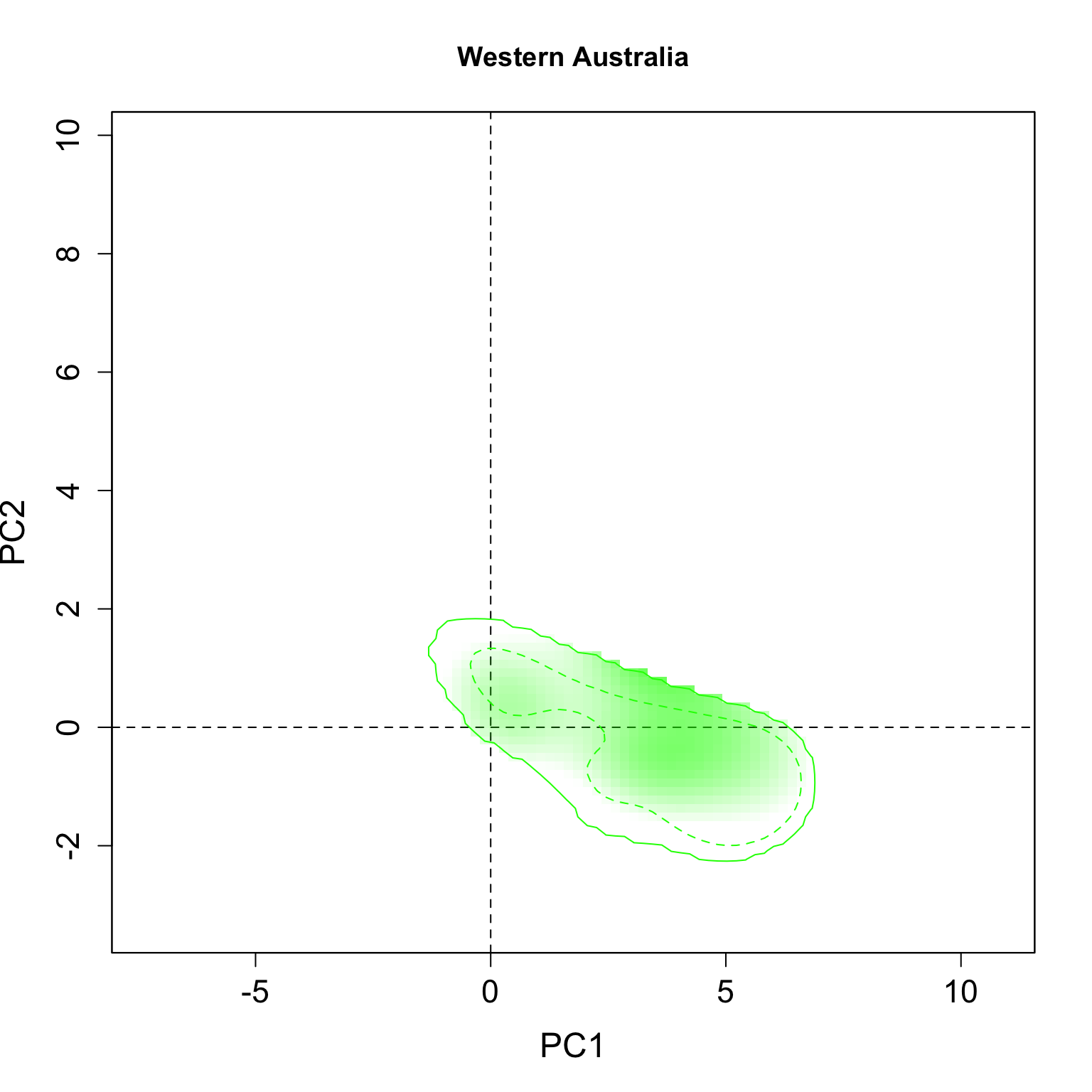
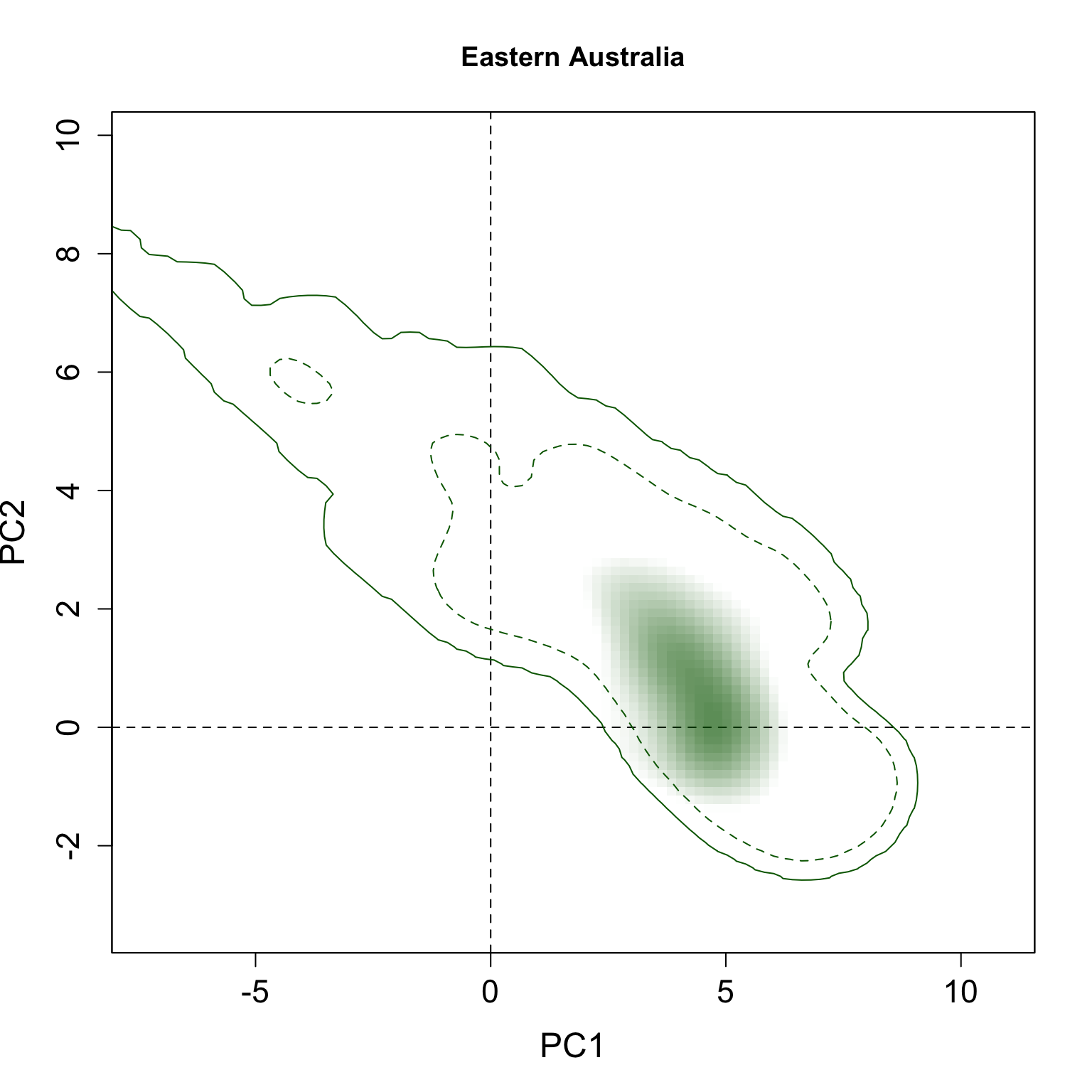
We applied this function here to plot all individual results per group. The continuous line represent the 100% of the available environmental background and the dashed line represents the 50% most common conditions.
for(i in 1:n.groups) {
  plot.niche.mod(z, name.axis1 = "PC1", name.axis2 = "PC2",
                 cor = F, corte,  contornar = FALSE,
                 densidade = TRUE, quantis = 3,
                 back = TRUE, x = g.colors[i], title = g.names[i], i)
}
Multiple niche plots
We also modified the same function to allow multiple regions/species plots.
plot.niche.all <- function(z, n.groups, g.names,
                           contornar = TRUE,
                           densidade = TRUE,
                           quantis = 10,
                           back = TRUE, title = "",
                           g.colors, n = 5,
                           cor1) {

  # Color func
  cor1 <- function(cores.i, n) {
    al <- seq(0,1,(1/n))
    cores <- numeric(length(n))
    for(i in 1:n) {
      corespar <- col2rgb(cores.i)/255
      cores[i] <- rgb(corespar[1, ], corespar[2, ],
                      corespar[3, ], alpha = al[i])
    }
    return(cores)
  }


  a <- list()
  for(i in 1:n.groups) {
    a[[i]] <- colorRampPalette(c("transparent", cor1(g.colors[i], n)),
                               alpha = TRUE)
  }

  xlim <- c(min(sapply(z, function(x){min(x$x)})),
            max(sapply(z, function(x){max(x$x)})))

  ylim <- c(min(sapply(z, function(x){min(x$y)})),
            max(sapply(z, function(x){max(x$y)})))

  image(z[[1]]$x, z[[1]]$y, as.matrix(z[[1]]$z.uncor), col = "white",
        ylim = ylim, xlim = xlim,
        zlim = c(0.000001, max(as.matrix(z[[1]]$Z), na.rm = T)),
        xlab = "PC1", ylab = "PC2", cex.lab = 1.5,
        cex.axis = 1.4)
  abline(h = 0, v = 0, lty = 2)
  box()

  if (back) {
    for(i in 1:n.groups) {
      contour(z[[i]]$x, z[[i]]$y, as.matrix(z[[i]]$Z), add = TRUE,
              levels = quantile(z[[i]]$Z[z[[i]]$Z > 0], c(0, 1)),
              drawlabels = FALSE,lty = c(1, 2),
              col = g.colors[i], lwd = 1)
    }
  }

  if (densidade) {
    for(i in 1:n.groups) {
      image(z[[i]]$x, z[[i]]$y, as.matrix(z[[i]]$z.uncor),
            col = a[[i]](100), add = TRUE)
    }
  }


  if(contornar){
    for(i in 1:n.groups) {
      contour(z[[i]]$x, z[[i]]$y, as.matrix(z[[i]]$z.uncor), add = TRUE,
              levels = quantile(z[[i]]$z.uncor[z[[i]]$z.uncor > 0],
                                seq(0, 1, (1/quantis)))[quantis],
              drawlabels = FALSE, lty = rev(c(rep(2,(quantis - 1)), 1)),
              col = rev(cor1(g.colors[i], quantis)),
              lwd = rev(c(rep(1, (quantis - 1)), 2)))
    }
  }

}
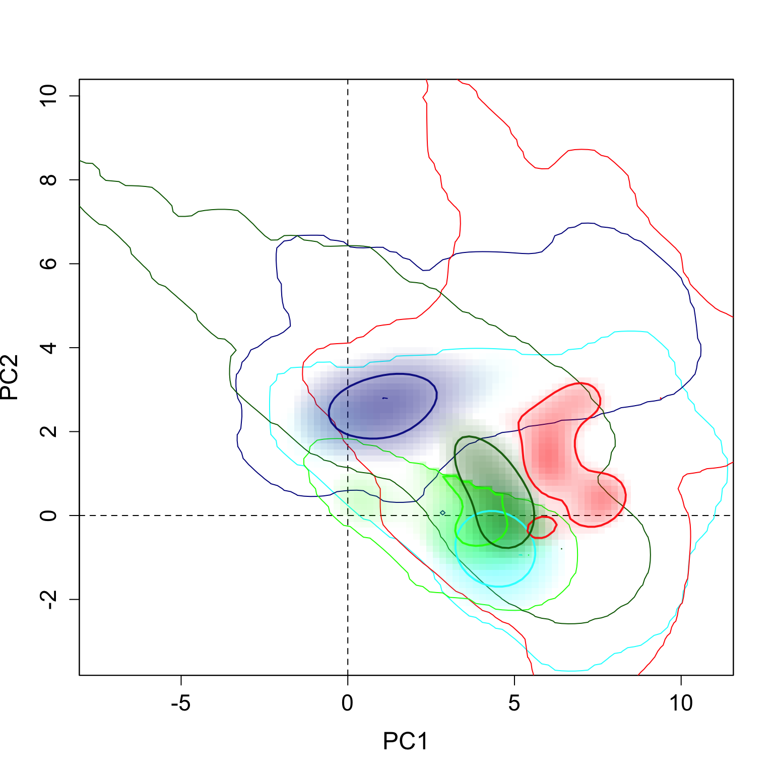
The results can be seen here. The strong contours represent the 5% highest values of density, and the thin lines represent 100% of the background available in each region.
plot.niche.all(z, n.groups, g.names,
               contornar = TRUE,
               densidade = TRUE,
               quantis = 10,
               back = FALSE, title = "",
               g.colors, n = 2,
               cor1)

plot.niche.all(z, n.groups, g.names,
               contornar = TRUE,
               densidade = TRUE,
               quantis = 10,
               back = TRUE, title = "",
               g.colors, n = 2,
               cor1)
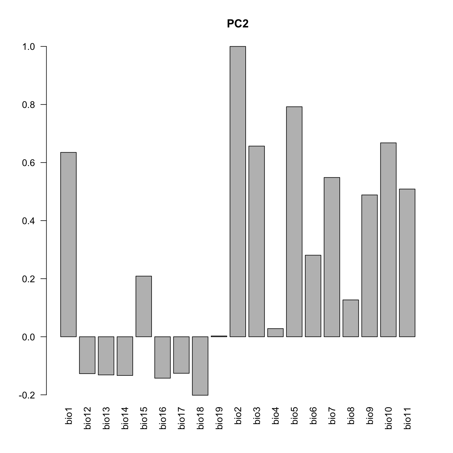
Below the loadings plot (contribution of the variables for each axis). Check the variable codes at http://www.worldclim.org/bioclim.
loadings <- cbind(cor(data.env, pca.cal$tab[,1]), cor(data.env, pca.cal$tab[,2]))
colnames(loadings) <- c("axis1", "axis2")
loadings <- loadings[c(1, 12:19, 2:11), ]

barplot(loadings[,1], las=2, main="PC1")

barplot(loadings[,2], las=2, main="PC2")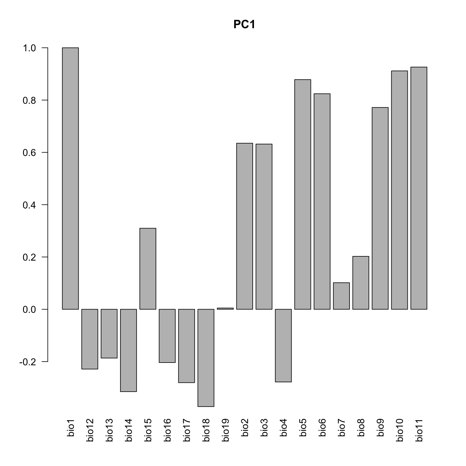
The arrows representing the contribution of each variable, directly on the environmental space.
contrib <- pca.cal$co
eigen <- pca.cal$eig
nomes <- numeric(19)
for(i in 1:19){
  nomes[i] <- paste('bio',i, sep="")
}
s.corcircle(contrib[, 1:2] / max(abs(contrib[, 1:2])),
            grid = F,  label = nomes, clabel = 1.2)
text(0, -1.1, paste("PC1 (", round(eigen[1]/sum(eigen)*100,2),"%)",
                    sep = ""))
text(1.1, 0, paste("PC2 (", round(eigen[2]/sum(eigen)*100,2),"%)",
                   sep = ""), srt = 90)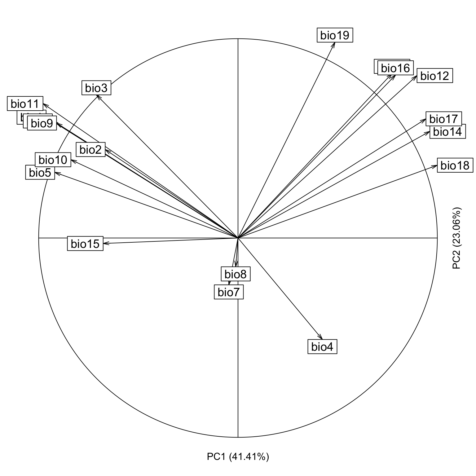
References
Aiello‐Lammens, M. E., Boria, R. A., Radosavljevic, A., Vilela, B., & Anderson, R. P. (2015). spThin: an R package for spatial thinning of species occurrence records for use in ecological niche models. Ecography, 38(5), 541-545.
Broennimann, O., Fitzpatrick, M. C., Pearman, P. B., Petitpierre, B., Pellissier, L., Yoccoz, N. G., & Guisan, A. (2012). Measuring ecological niche overlap from occurrence and spatial environmental data. Global Ecology and Biogeography, 21(4), 481-497.
Hanski, I., & Cambefort, Y. (Eds.). (2014). Dung beetle ecology. Princeton University Press.